Authors: (in alphabetical order) Enrico Antonini, Siddharth Krishna, Daniele Lerede
Contributors: Heba Badawy, Jacek Bendig, Kristijan Faust, Fabrizio Finozzi, Priya Goli Vamsi, Madhukar Mishra, Maximillian Parzen, and Luis Prieto
Funder: Breakthrough Energy
Acknowledgements: The authors would like to thank the following individuals for their valuable feedback during the preparation of this report (listed alphabetically): Oscar Dowson (JuMP), Ivet Galabova (HiGHS), Julian Hall (HiGHS), Lennart Lahrs (Gurobi), Matthias Miltenberger (Gurobi), Mark Turner (MIPLIB), and Filippo Zanetti (HiGHS).
Resources: The complete report, benchmark instances, and metadata are available on Zenodo
Abstract
This report presents the 2025 results of the Open Energy Benchmark initiative, a transparent and reproducible benchmarking effort evaluating optimization solvers on realistic, community-contributed energy system models. The benchmark compares four open-source solvers (CBC, GLPK, HiGHS, and SCIP) and a proprietary baseline (Gurobi) across a diverse set of LP and MILP problems originating from 13 modeling frameworks. Using 213 benchmark problems, the report evaluates solver performance in terms of runtime, success rate, and scalability under standardized computational settings. The analysis highlights how solver capabilities vary depending on problem class, model formulation, and problem scale, while also exploring the evolution of solver performance over time and the computational challenges associated with increasingly large and complex energy planning models. The purpose of this report is not to identify a single "best" solver or produce a universal ranking of solver packages. Solver performance depends strongly on the characteristics of the optimization problem, modeling framework, configuration choices, and user requirements. Instead, the benchmark is intended as an educational and diagnostic resource that helps energy modelers better understand solver behavior, helps solver developers identify opportunities for improvement, and helps funding organizations identify areas where investments in open-source optimization software can have the greatest impact.
Key Findings
- Open-source optimization solvers for energy system modeling continue to improve in both runtime and reliability, but substantial performance gaps remain compared to proprietary solvers, particularly for large and complex models.
- Large-scale MILP problems remain especially challenging for open-source solvers, with significant scalability limitations and frequent timeouts at higher problem sizes.
- Solver performance depends strongly not only on problem size, but also on mathematical formulation, modeling framework, and algorithm selection.
- Open and reproducible benchmarking provides valuable domain-specific feedback for both energy modelers and solver developers and can help accelerate improvements in open-source and proprietary optimization tools.
Introduction
The transition toward decarbonized energy systems relies on advanced computational models to plan capacity expansion and optimize operational dispatch. As modelers strive to integrate emerging technologies across both supply and demand, enable faster decision-making for short-term operations and long-term planning, and account for the impacts of climate change and socio-economic development, the scale and complexity of the underlying mathematical optimization problems have grown substantially. These models predominantly take the form of Linear Programming (LP) and Mixed-Integer Linear Programming (MILP) problems, often containing millions of variables and constraints.
Because of the scale of such problems, the performance of the optimization solver, which is tasked with finding the most cost-effective system configurations, has become a primary bottleneck in energy system planning. Runtime and memory usage dictate practical usability; extended solve times and inefficient memory usage restrict the number of scenarios that can be evaluated and the level of spatial or temporal resolution that can be included. When computational constraints limit scenario analysis, modelers cannot fully explore the impacts and uncertainties associated with technology costs, policy decisions, or climate change, which reduces the robustness of the resulting energy system planning.
For years, proprietary commercial solvers have served as a performance baseline, successfully processing models with millions of variables. The computational limits of open-source solvers constrain the scale of models that can be solved, often forcing modelers to compromise on detail to achieve a solution without commercial licenses. However, the open-source solver ecosystem has seen steady advancements in recent years, increasingly pushing the boundaries of what is computationally tractable. To accurately navigate this evolving landscape and identify the areas where open-source solvers need improvement, energy modelers, solver developers, and funding stakeholders require transparent, reproducible, and domain-specific performance data.
This report presents a quantitative assessment of five solver packages: four open-source options (CBC, GLPK, HiGHS, and SCIP) and one proprietary tool (Gurobi) used as a baseline. Leveraging the open-source benchmarking infrastructure developed by Open Energy Transition and hosted at the Open Energy Benchmark platform, we evaluate the capabilities of these solver packages on realistic, community-contributed energy models. We evaluate performance based on both the average runtime and the fraction of successfully solved problems within established time and memory limits (success rate). To ensure a standardized, out-of-the-box comparison, all solver packages were executed using their default configuration options, though users should note that selecting specific algorithms or tuning settings can improve performance.
The purpose of this report is not to identify a universally "best" solver or provide a definitive ranking of solver packages. Solver performance depends strongly on the characteristics of the optimization problem, the modeling framework, the selected algorithms, and user-specific requirements. Instead, the benchmark is intended as an educational and diagnostic resource that helps energy modelers better understand solver behavior, helps solver developers identify areas for improvement, and helps funding organizations identify opportunities to accelerate the development of open-source optimization software.
The next sections present an overview of the benchmarking results while details on the problems, solvers, and computational infrastructure are available in the “Benchmark details” section at the end.
Results
Results by problem class and number of variables
The benchmark suite is divided between LP and MILP problems, reflecting the different mathematical requirements of models with capacity expansion (LP) and discrete operational or investment decisions (MILP). As shown in the size distribution (Figure 1, panels (a) and (b)), LP problems constitute the bulk of the largest cases in our benchmark suite with almost 60 problems in the 106 to 108 variable range. In contrast, MILP problems are generally smaller in scale. The majority of MILP problems in our benchmark suite fall within the 104 to 105 variable range, with just 2 exceeding 106 variables. It should also be noted that not all solver packages are equally suited for both problem types (e.g., SCIP specializes in MILPs while GLPK struggles with large-scale MILPs), an inherent specialization that should be considered when comparing aggregate performance metrics across the suite.
When evaluating the percentage of problems successfully solved within the established time and memory limits (Figure 1, panels (c) and (d)), different solver capabilities become visible across problem classes and scales. Gurobi, used here as a proprietary baseline, maintains high success rates across both problem types (generally between 60% to 80%) and provides a reference point for measuring how much room remains for improvement in open-source solvers.
Among the open-source solvers, differences emerge based on the problem type and scale. For LP problems, HiGHS demonstrates the highest success rate. For MILP problems, HiGHS and SCIP generally outperform CBC, with SCIP showing the highest success rate among the open-source options in the 105 to 106 variable range, while GLPK consistently lags behind across all problem sizes. The results also show a decrease in success rate for all open-source options as LP problem sizes cross the 1 million variable threshold, highlighting the current scalability barrier and the scale range where further algorithmic progress would have the largest impact.
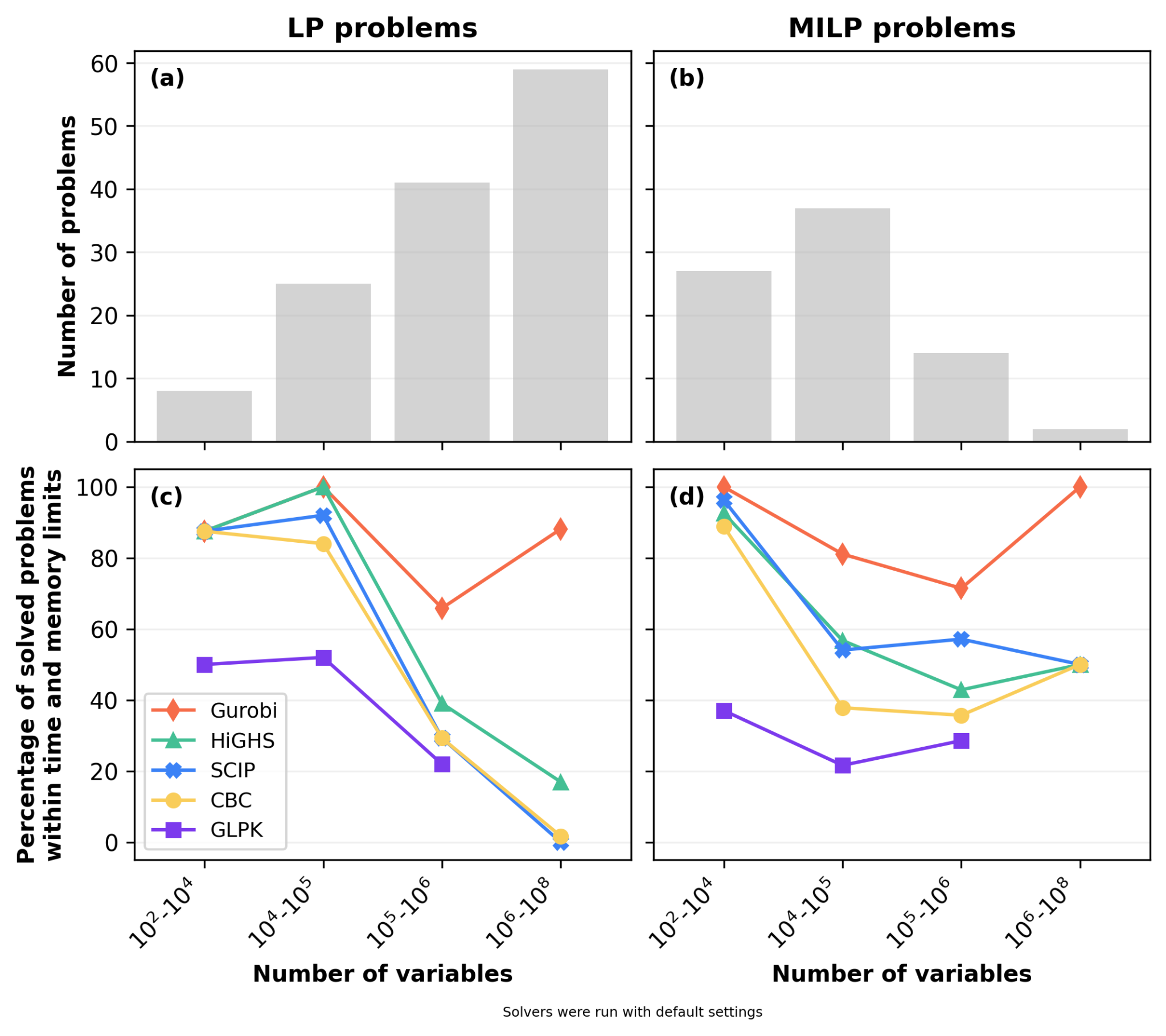
Figure 1: Distribution of benchmark problems and solver success rates by problem size. Panels (a) and (b) display the absolute number of Linear Programming (LP) and Mixed-Integer Linear Programming (MILP) problems, categorized by the number of variables. Panels (c) and (d) illustrate the percentage of these problems successfully solved within the established time and memory limits by each solver across the respective size categories. Problems with less than one million variables were run on virtual machines with 7 GiB RAM and a 1-hour timeout, whereas problems with more than one million variables were run on virtual machines with 124 GiB RAM and a 24-hour timeout.
Beyond success rate, the average computational runtime required to solve these models is another important measure of solver performance and real-world applicability (Figure 2, panels (a) and (b)). To provide a balanced assessment of runtime across different problem configurations, we utilize the shifted geometric mean (SGM), where the runtime of unsolved problems (timeouts or errors) is set equal to the time limit.
At the smallest scales (102 to 104 variables), runtime differences across solvers are relatively minor for LP problems, with Gurobi, HiGHS, SCIP, and CBC all solving problems in under a minute on average. However, as the problem scale increases, runtime trajectories diverge. For LP problems exceeding 105 variables, Gurobi maintains a relatively lower average runtime, routinely solving these larger problems in under an hour, which establishes the target runtime for open-source alternatives. Conversely, the open-source solvers experience an increase in average runtime, approaching the 24-hour timeout ceiling for problems with more than 106 variables. In the MILP domain, there is room for improvement for open-source solvers even at smaller scales, with the proprietary baseline frequently finding solutions orders of magnitude faster than its open-source counterparts.
To quantify this runtime difference, we also analyze the relative speed of the solvers across different size bins (Figure 2, panels (c) and (d)). When comparing the open-source options to the fastest available solver (Gurobi), a quantifiable gap is evident. In both the LP and MILP categories, the open-source tools can be anywhere from a few times to over a hundred times slower than the proprietary baseline, depending on the specific problem scale and type, showing where future development can yield the highest speedups. Among the open-source suite, HiGHS consistently emerges as the most time-efficient option for LP problems, particularly in the 104 to 106 variable range where it outpaces SCIP, CBC, and GLPK. However, for larger problems (106 variables and above), the relative runtime becomes influenced by timeouts. Because open-source solvers frequently fail to return solutions within the time limits at these scales, their average runtimes hit the penalization ceiling.
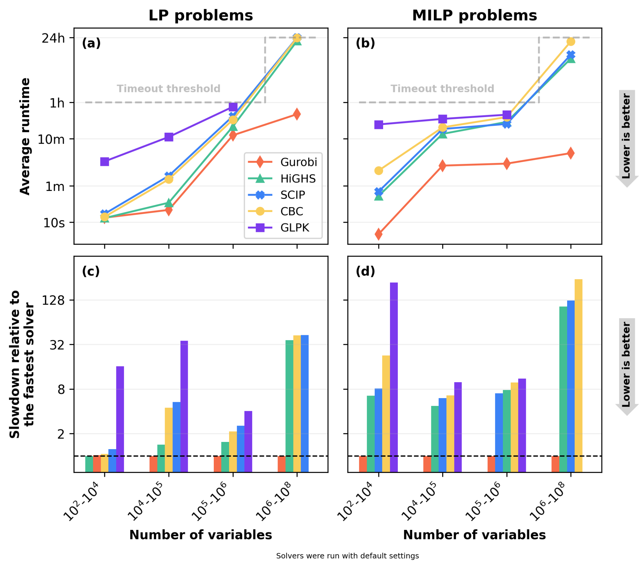
Figure 2: Average computational runtime and relative slowdown across varying problem sizes. Panels (a) and (b) display the absolute average runtime for LP and MILP problems, calculated as the shifted geometric mean with a penalty of twice the timeout threshold for unsolved problems. Panels (c) and (d) illustrate the relative computational slowdown of each solver compared to the fastest solver in that specific size category.
Results by modeling framework
The benchmark problems originate from 13 modeling frameworks, and these differences in model origin may influence their underlying mathematical structure, including problem size, sparsity patterns, numerical conditioning, and the balance between continuous and discrete decisions. To understand this impact, we evaluated solver performance across these distinct frameworks, analyzing both the structural characteristics of their typical models and the resulting computational outcomes. However, because the available benchmark problems are community-contributed, they may not perfectly represent the entire spectrum of models each framework is capable of generating; therefore, these results offer indicative trends rather than universal conclusions.
Figure 3 illustrates the variations across frameworks in the number and size of benchmark problems, as well as the corresponding solver success rates and average runtimes. For this analysis, modeling frameworks contributing five or fewer problems (DCOPF, IESA-Opt, PowerModels, and ZEN-garden) have been grouped into a single category designated as "Others." Among the individually tracked frameworks, SWITCH is primarily represented by smaller problems, whereas PyPSA and TEMOA feature problems that frequently exceed one million variables. PyPSA accounts for the largest share of the benchmark problems, which proportionally influences the overall performance averages for larger problems.
The performance data indicates that while high success rates can be achieved across almost all frameworks when using any available solver, the capabilities of open-source tools are much more sensitive to a framework's typical problem scale and formulation. Open-source solvers achieve near-perfect success rates on the smaller models from OEMOF, but their success rate drops on the larger or more complex problems generated by GenX and PyPSA. Furthermore, the varying success rates among frameworks with similar problem sizes demonstrate how specific mathematical formulation choices can create computational bottlenecks independent of raw variable count. This points to structural sensitivities within certain modeling approaches that open-source developers can target for future algorithm improvements.
This sensitivity is also apparent when examining average runtime. While all solvers perform similarly on frameworks with smaller median variable counts (such as SWITCH or ETHOS.FINE), a measurable divergence emerges as problem scale increases. For frameworks like TEMOA and TIMES, the best open-source solver requires an order of magnitude more computational time than the overall best solver, underscoring the performance gap that open-source tools must close to handle large models efficiently.
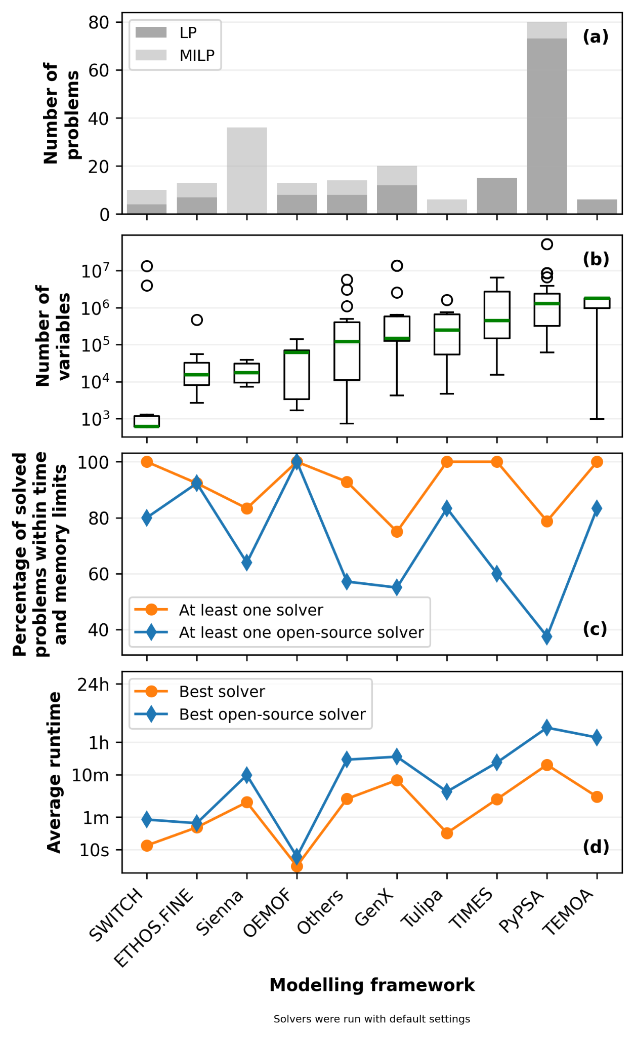
Figure 3: Solver performance and problem characteristics categorized by modeling framework. Frameworks on the x-axis are sorted in ascending order by the median number of variables. Panel (a) shows the number of benchmark problems contributed by each framework. Panel (b) displays the distribution of problem sizes, with the green line indicating the median. Panel (c) illustrates the percentage of problems successfully solved within time and memory limits, and panel (d) shows the average runtime, calculated as the shifted geometric mean with a penalty of twice the timeout threshold for unsolved problems. The “Others” category groups modeling frameworks contributing five or fewer problems, which are DCOPF, IESA-Opt, PowerModels, and ZEN-garden.
Solver performance evolution
We analyzed the historical performance of solver packages by benchmarking successive software releases across our standardized problem set from 2022 to 2025. Both CBC and GLPK are omitted from this historical analysis. CBC is removed due to a lack of sufficient historical data, as only two years (2023 and 2024) of releases were available to track. GLPK is also excluded because its most recent major update occurred in 2020, meaning its performance has remained static during this period.
For this specific analysis of performance evolution, we restricted the benchmark suite to problems with fewer than 1 million variables, which means that solver improvements that specifically target larger problems are not tracked by this analysis. Furthermore, because we evaluated only default configurations, any performance gains dependent on specific algorithms or non-default parameter settings may still occur but are not captured here. Finally, to manage computational costs, all evaluations currently rely on a single random seed. Because solver performance can exhibit significant variability depending on the initial seed, minor version-to-version changes should be interpreted with caution, as results could shift under different seed conditions.
The performance evolution data (Figure 4) shows divergent development paths across the solver ecosystem. SCIP shows little change in either the fraction of successfully solved problems or average computational runtime over the tracked period. In contrast, the baseline proprietary solver demonstrates active algorithmic progress. Gurobi has maintained its high success rate while consistently reducing its average runtime year-over-year, showing a decrease of approximately 3% relative to its 2022 baseline.
The most noticeable evolution in open-source solver packages is observed in HiGHS. Despite a minor dip in success rate in 2023, HiGHS has improved over time, showing a roughly 2 percentage point increase in the fraction of solved problems by 2025 compared to its initial baseline. Concurrently, HiGHS has achieved a 3% reduction in average runtime, matching the relative pace of Gurobi’s speed improvements. It is worth noting that performance regressions (like the 2023 dip) may occur when developers implement stricter numerical handling, or they may simply reflect an updated algorithm's sensitivity to a specific model set. Overall, this data indicates that while some open-source tools have shown little change in speed or success rate on this specific set of energy problems, HiGHS is actively improving its capabilities and narrowing the gap with proprietary optimization software.
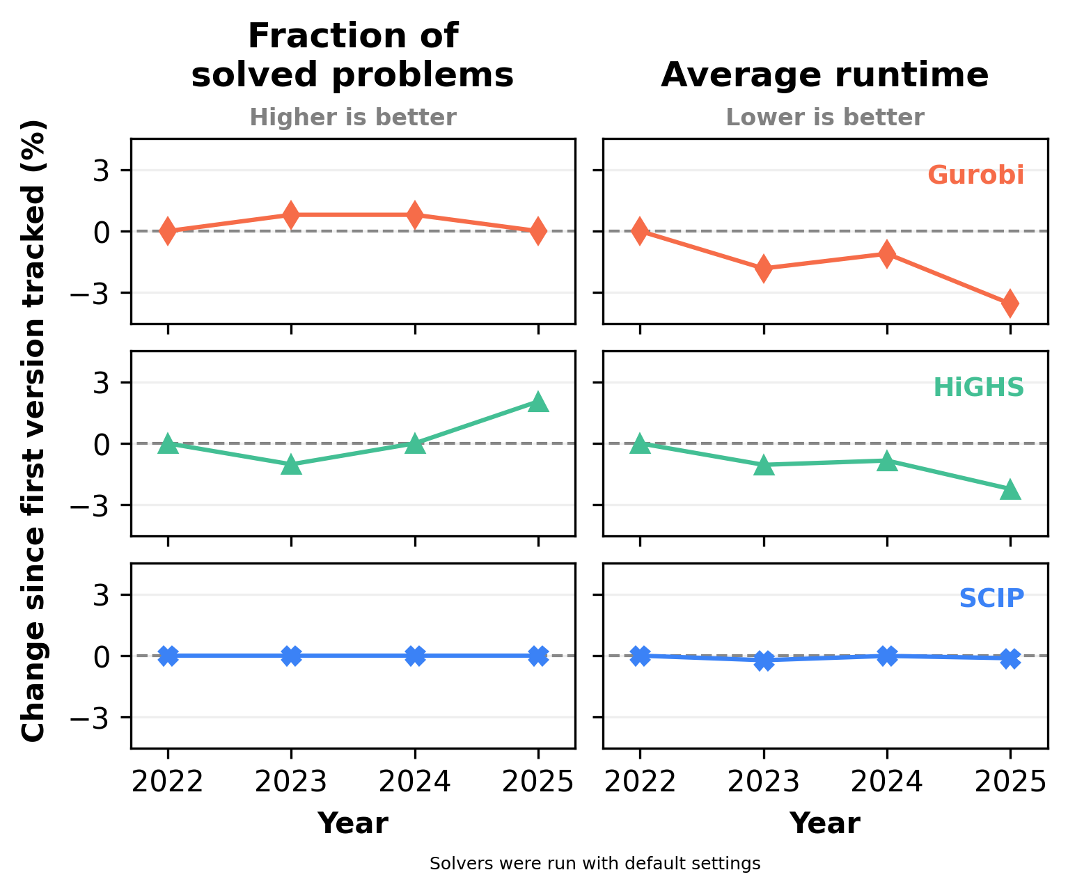
Figure 4: Evolution of solver performance over time (2022–2025) on benchmark problems with fewer than 1 million variables. The left panels display the percentage point change in the fraction of successfully solved problems relative to the first tracked version of each solver. The right panels show the percentage change in average computational runtime relative to the first tracked version. CBC is removed from the analysis due to a lack of sufficient historical data, as only two years (2023 and 2024) of releases were available to track. GLPK is also excluded from this figure as it is only available in a single version from 2020.
Scaling barriers in a PyPSA electricity model
To illustrate how solver runtime changes with increasing spatial and temporal resolution, Figure 5 presents results for a case study of Germany’s electricity system built using PyPSA-Eur, modeling overnight capacity expansion to 2050 without transmission expansion optimization. We consider cases without unit commitment (panel a), which result in LP problems, and cases with unit commitment applied to conventional generators (panel b), which lead to MILP problems.
For the LP formulation, computational complexity scales with both spatial and temporal resolution. However, assessing how far spatial resolution can be increased within computational limits is a common question in energy system modeling; therefore, we focus on the effect of increasing spatial resolution in the LP cases. In contrast, for the MILP formulation, temporal resolution has a greater impact due to the inclusion of unit commitment decisions. Specifically, unit commitment introduces inter-temporal constraints (such as minimum up/down times, startup and shutdown decisions, and associated costs) that link decisions across time, transforming a smooth, convex problem into a combinatorial optimization problem. Accordingly, we present solver runtime as a function of temporal resolution for the MILP cases.
For LP problems, all solvers reach a solution within the time limits up to 8 nodes (approximately 1.7×10⁶ variables). CBC is generally the slowest solver and is the first to reach the 24-hour time limit at 10 nodes, followed by HiGHS at 14 nodes, as the problem approaches approximately 2.8×10⁶ variables. For MILP problems, solvability barriers arise at much smaller problem sizes: SCIP, HiGHS, and CBC reach time limits with only around 3.2×10⁴ variables at a temporal resolution of 24 hours. Note that SCIP is shown only for MILP, as it is better suited to mixed-integer problems, while GLPK is not considered in this scaling analysis.
Panels (c) and (d) show the number of variables for all problems. In LP problems, the number of variables grows linearly with spatial resolution. In MILP problems, the number of variables would also grow linearly with spatial resolution (if varied independently), but in this analysis we observe an exponential growth with temporal resolution.
It is important to note that this case study may not be fully representative of the entire benchmark set. In particular, we observe that some MILP problems of substantially larger size can still be solved within the same time and memory limits. The performance limitations highlighted here may therefore reflect specific structural characteristics of the PyPSA framework rather than general properties of all energy system MILPs. At the same time, the use of a consistent problem generation script across all the problems of this scaling analysis ensures comparability and may help reveal structural features that could remain hidden in the full benchmark set with heterogeneous model frameworks, scenarios, and resolution choices.
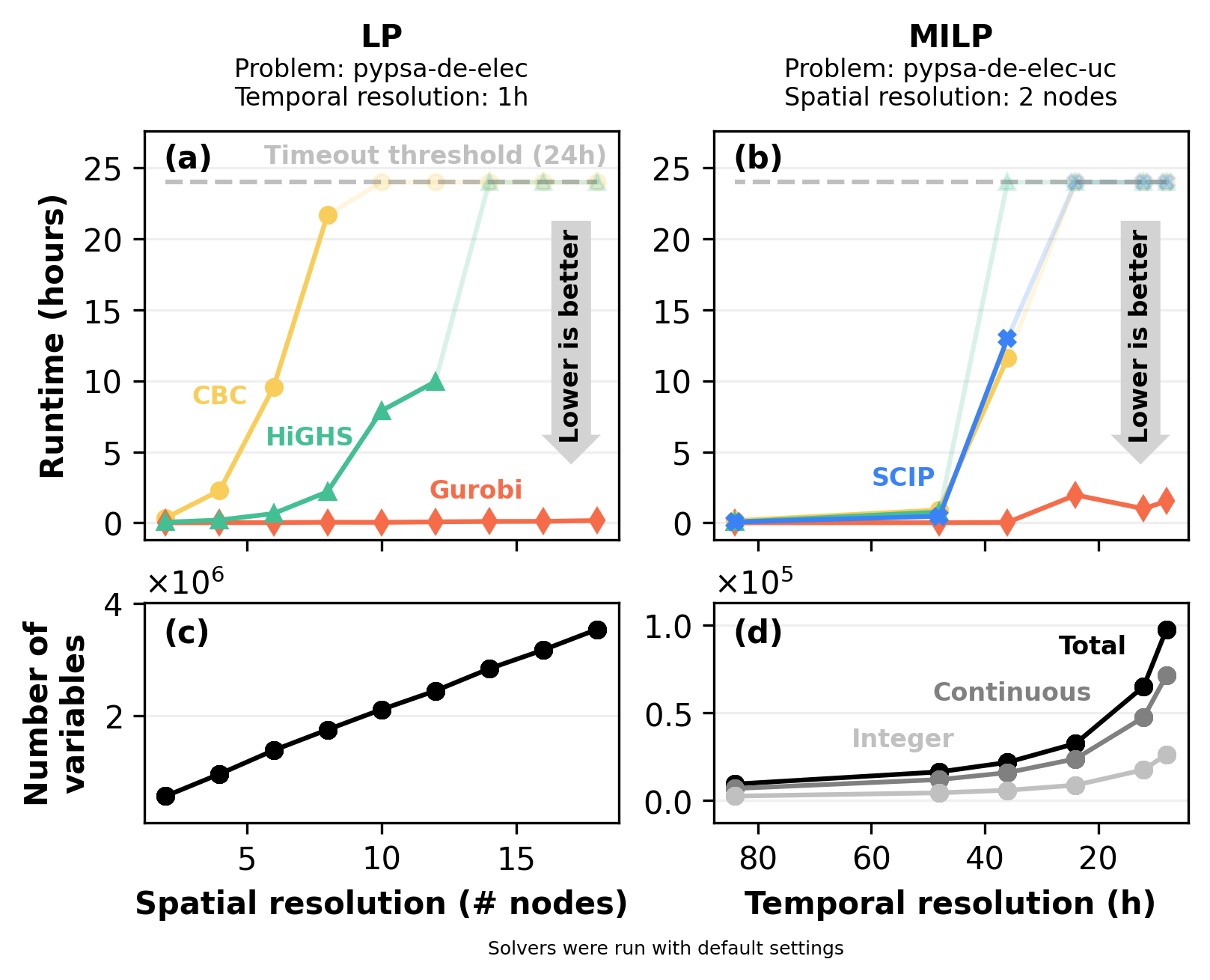
Figure 5: Solver runtimes and problem size for a PyPSA electricity-only case study for Germany with a zero-emissions 2050 target. Panel (a) and (b) show the runtime for the LP (without unit commitment) and MILP (with unit commitment) formulations, respectively. Panels (c) and (d) show how the number of variables grows with spatial and temporal resolution, respectively.
Solver algorithm selection and the HiPO interior-point method
Beyond comparing default solver configurations, we performed a complementary study on how algorithm selection can influence solver performance on large-scale energy system models. The study, which is briefly summarized here, evaluated a new implementation of the interior-point method (HiPO) in HiGHS on LP benchmark problems. Its performance was compared against the existing HiGHS algorithms, namely the previous implementation of the interior-point method (IPX) and the dual simplex solver. The results of Gurobi using its default configuration from the benchmark run presented above was used as a proprietary baseline.
The results showed that algorithm choice can significantly affect computational performance depending on the structure and scale of the optimization problem. The new HiPO interior-point implementation significantly extended the scale of LP energy system models that can be solved using open-source tools. Across the benchmark suite, HiPO increased the number of problems solvable by open-source solvers by 7% and solved models with millions of variables up to 15 times faster than the existing HiGHS simplex and IPX, particularly for problems between 105 and 107 variables.
Figure 6 illustrates these findings for the same representative LP problems as from the previous section, derived from a PyPSA electricity model for Germany. The figure shows how solver runtime evolves as the spatial resolution of the model increases from 2 to 60 network nodes, corresponding to problem sizes ranging from approximately 0.5 to more than 10 million variables. While the HiGHS simplex and IPX implementations reach the 24-hour timeout threshold at 14 and 20 nodes, respectively, HiPO can solve instances up to 50 nodes and maintains lower runtimes across most of the resolution range.
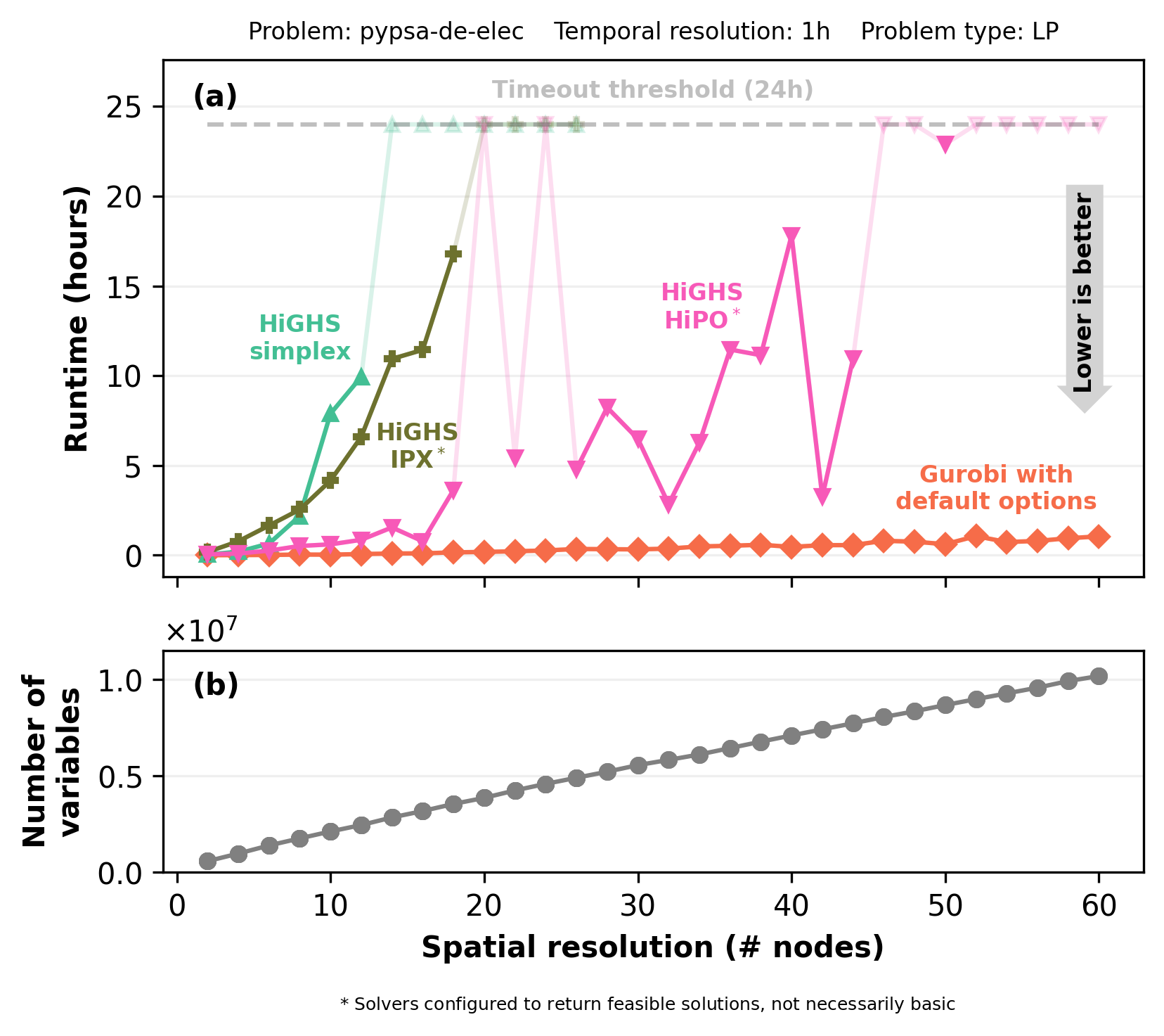
Figure 6: Solver runtimes and problem size for a PyPSA electricity-only case study for Germany with a zero-emissions 2050 target. Panel (a) shows solver runtime for different HiGHS algorithms and Gurobi. Panel (b) shows the corresponding growth in the number of variables. Solvers marked with an asterisk were configured to return feasible solutions, not necessarily basic solutions.
The study also highlighted the importance of crossover behavior and the distinction between feasible and basic solutions (additional details are included in the referenced study). Simplex methods naturally return basic solutions, while interior-point methods typically return feasible interior solutions unless an additional crossover phase is performed to recover a simplex basis. Note that in the referenced HiPO study we evaluated Gurobi using its default configuration, which runs multiple algorithms in parallel, including simplex and barrier interior-point methods with crossover, taking advantage of all available CPU cores and always returning a basic solution. By contrast, the HiPO and IPX runs in HiGHS were performed with an optional crossover, meaning that they returned feasible interior solutions that were not always basic. As a result, the interior-point results from Gurobi and HiGHS should not be interpreted as directly comparable. A more comparable configuration in Gurobi would require setting “SolutionTarget=1”, which removes the requirement for a basic solution and allows crossover to be skipped if the interior-point solution meets the solution accuracy thresholds.
Conclusions
The benchmarking of 213 energy system optimization models reveals a detailed picture of current solver capabilities, highlighting both the progress of open-source tools and the remaining performance gaps compared to proprietary alternatives. Based on the Open Energy Benchmark data, the key findings are:
- The Scale Barrier for Open-Source: Open-source solvers face a critical scalability limit, typically around the 1 million variable threshold. While tools like HiGHS perform well on smaller continuous problems, their success rates drop significantly, and runtimes hit hard computational limits as problems scale into the millions of variables.
- The MILP Challenge: The performance gap is most pronounced for MILP problems. The inclusion of discrete decisions amplifies the computational burden, causing open-source solvers to run up to 100 times slower than the proprietary baseline, or to time out entirely, even at problem sizes between 105 and 106 variables.
- Sensitivity to Mathematical Formulation: Solver success is heavily dependent on the specific modeling framework used, not just the raw problem size. Open-source solvers achieve high solve rates on certain frameworks (e.g., OEMOF) but experience high failure rates on others with denser or more complex mathematical formulations (e.g., PyPSA), highlighting the importance of structural choices in model design and identifying specific formulation patterns that challenge current open-source algorithms.
- Ongoing Progress in Open-Source Solvers: The performance evolution study demonstrates some progress by open-source tools, notably HiGHS, on our benchmark set. Because we only tested historical solver versions on the problems with fewer than 106 variables, advances on large problems were not measured. Recent developments such as HiPO are also not captured because our methodology runs solvers with default configurations. However, the complementary HiPO study demonstrates that new algorithmic developments can yield substantially larger performance gains, such as a 7% increase in the number of energy planning problems solvable by open-source tools and up to 15 times faster runtimes for models with millions of variables.
Ultimately, while proprietary solvers remain necessary for the largest energy models, the active development of tools like HiGHS proves that the frontier of open-source capabilities is steadily expanding. Advancing this frontier requires continuous feedback between modelers and solver developers. The Open Energy Benchmark platform facilitates this by providing a diagnostic space where solver developers can identify specific weaknesses and target improvements for upcoming releases. To keep this resource comprehensive, Open Energy Transition invites the modeling community to contribute additional LP and MILP problems following the guidelines available at the Open Energy Benchmark website. By submitting models from underrepresented frameworks or large-scale instances specifically designed to stress-test algorithms, the community can directly help shape and accelerate open-source solver development.
Benchmark details
Number and types of problems
The benchmark draws on a broad collection of energy system optimization problems available through the Open Energy Benchmark platform. Each problem is generated by a given combination of model framework, scenario, and resolution. The model framework is the software and mathematical framework used to formulate optimization problems. The scenario specifies the system under study and its assumptions, such as geographic scope, temporal scope, sectoral scope, available technologies, technology costs, policy constraints, and other boundary conditions. The resolution describes the spatial and temporal granularity used in the scenario.
In total, the benchmark contains 213 problems. Of these, 133 are LP problems and 80 are MILP problems. This provides coverage of both continuous planning formulations and models that include discrete investment or operational decisions.
The problems originate from 13 modeling frameworks, although their representation is uneven, as detailed in Table 1. PyPSA contributes the largest number with 80, followed by Sienna with 36 and GenX with 20. A middle group includes TIMES (15), ETHOS.FINE (13), and OEMOF (13), while SWITCH contributes 10. Smaller contributions come from TEMOA (6), Tulipa (6), PowerModels (5), DCOPF (4), IESA-Opt (3), and ZEN-garden (2).
This composition gives the benchmark a wide methodological spread, but it also means that some frameworks and problem classes are represented more densely than others. As a result, aggregate benchmark results are informative about the available test set, while framework-specific conclusions should be interpreted in light of the number and diversity of problems contributed by each framework.
| Modeling framework | Problems |
|---|---|
| PyPSA | 80 |
| Sienna | 36 |
| GenX | 20 |
| TIMES | 15 |
| ETHOS.FINE | 13 |
| OEMOF | 13 |
| SWITCH | 10 |
| TEMOA | 6 |
| Tulipa | 6 |
| PowerModels | 5 |
| DCOPF | 4 |
| IESA-Opt | 3 |
| ZEN-garden | 2 |
Table 1: Summary of benchmark problems categorized by originating modeling framework.
To evaluate solver performance across this diverse dataset, problems are categorized by their scale. As illustrated in Figure 7, there is a strong, nearly linear relationship between the number of variables in a problem and both the number of non-zero elements (Panel a, R2=0.981) and the number of constraints (Panel b, R2=0.984). Because these structural dimensions scale so predictably with the variable count, grouping the benchmark problems by the number of variables serves as a robust and representative proxy for overall problem size and mathematical complexity.
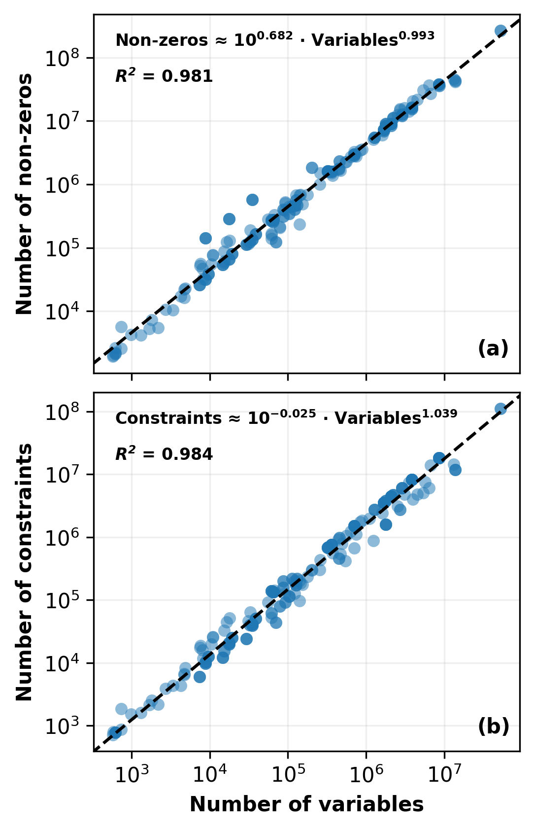
Figure 7: Relationship between problem scale characteristics across the benchmark suite. Panel (a) shows the number of non-zero elements scaling nearly linearly with the number of variables. Panel (b) illustrates a similar linear scaling between the number of constraints and the number of variables.
Solver packages
To provide a comprehensive assessment of the optimization landscape, the benchmark evaluates one proprietary solver package (Gurobi) alongside four open-source alternatives (CBC, GLPK, HiGHS, and SCIP), all listed in Table 2. GLPK is only available in a single version from 2020 and is included to represent legacy open-source capabilities, as it has not received major updates since that time. Conversely, Gurobi, HiGHS, and SCIP have maintained active development cycles, allowing the benchmark to capture their annual progress from 2022 through 2025.
All solver packages were executed using their default configuration options with a few exceptions (Table 3), though selecting specific algorithms or tuning settings can improve performance. In practice, solver packages are generally expected to choose an appropriate algorithm automatically for the problem at hand, using, for example, simplex or interior-point methods for LP problems and branch-and-bound or branch-and-cut variants for MILP problems, depending on the capabilities of the package. This approach ensures a standardized, out-of-the-box comparison that reflects the baseline performance most modelers will experience, without relying on problem-specific algorithmic tuning. The only exceptions to this rule are the enforcement of a fixed random seed to a value of 0 (to guarantee reproducibility) and setting a uniform duality gap tolerance of 10-4 for all MILP problems, which allows solvers to terminate in a reasonable timeframe once they find a high-quality solution.
It should be noted that not all solver packages are equally suited for both LP and MILP problems. Some frameworks rely on distinct underlying components; for example, CBC and SCIP are primarily MILP solvers that delegate continuous problems to separate LP backends (CLP and SoPlex, respectively). Because of its specific architecture, SCIP is optimized for mixed-integer programming but less efficient for pure LPs. Conversely, GLPK faces a different limitation, frequently struggling with large-scale MILPs. This inherent specialization should be considered when comparing aggregate performance metrics across the entire suite.
While the present report focuses on default settings, we performed a separate study evaluating different solver variants and configurations for the HiGHS solver package, specifically focusing on a new implementation of interior-point method (HiPO).
| Solver package | Licensing model | Version | Release Year |
|---|---|---|---|
| CBC | Open source | 2.10.11 | 2023 |
| CBC | Open source | 2.10.12 | 2024 |
| GLPK | Open source | 5.0 | 2020 |
| Gurobi | Proprietary | 10.0.0 | 2022 |
| Gurobi | Proprietary | 11.0.0 | 2023 |
| Gurobi | Proprietary | 12.0.0 | 2024 |
| Gurobi | Proprietary | 13.0.0 | 2025 |
| HiGHS | Open source | 1.5.0.dev0 | 2022 |
| HiGHS | Open source | 1.6.0.dev0 | 2023 |
| HiGHS | Open source | 1.9.0 | 2024 |
| HiGHS | Open source | 1.12.0 | 2025 |
| SCIP | Open source | 8.0.3 | 2022 |
| SCIP | Open source | 8.1.0 | 2023 |
| SCIP | Open source | 9.2.0 | 2024 |
| SCIP | Open source | 10.0.0 | 2025 |
Table 2: Overview of the solver packages evaluated, including the specific versions and release years tracked in the benchmark.
| Option | Gurobi | HiGHS | SCIP | CBC | GLPK |
|---|---|---|---|---|---|
| Algorithm selection | Auto (Primal/Dual simplex, Barrier interior-point) | Auto (Primal/Dual simplex, IPX interior-point) | Branch-and-cut + LP solver (SoPlex, typically dual simplex) | Branch-and-cut (CLP simplex for LP relaxations) | Branch-and-bound + simplex |
| Solution type (LP) | Basic (or basic after crossover) | Basic (simplex) or non-basic (IPM) | Basic (SoPlex) | Basic (CLP) | Basic |
| Crossover | Auto (enabled if barrier) | Auto (run_crossover = choose) |
N/A | N/A | N/A |
| Barrier/IPM tolerance | 1e-8 | 1e-8 | N/A | N/A | N/A |
| Primal feasibility tolerance | 1e-6 | 1e-7 | 1e-6 | 1e-6 | 1e-6 |
| Dual feasibility tolerance | 1e-6 | 1e-7 | 1e-6 | 1e-6 | 1e-6 |
| Threads | All available cores | All available cores | 1 | 1 | 1 |
| MIP gap | 1e-4 | 1e-4 | 1e-4 (default = 0) | 1e-4 (default = 0) | 1e-4 (default = 0) |
| Random seed | 0 | 0 (default = not fixed) | 0 | 0 (default = time-based) | 0 (default = not fixed) |
| Notes | Uses branch-and-cut for MILPs with simplex, typically dual, for node relaxations; barrier uses crossover by default | Uses branch-and-cut for MILPs with simplex, typically dual, for node relaxations; IPM may skip crossover | MILP-focused solver; LP handled by SoPlex; limited parallelism | Limited cut generation and parallelism; relies on CLP for LP solves | Legacy solver; limited performance on large-scale MILPs |
Table 3: Overview of the solver options adopted in the benchmarking process. Parameters modified from their native default values are highlighted in orange; all other listed options represent the standard default settings.
Benchmark execution
All benchmark runs were carried out on Google Cloud virtual machines using a custom benchmarking infrastructure developed with Python and OpenTofu for the Open Energy Benchmark, designed to be open, transparent, and reproducible. Running the benchmark on publicly available cloud virtual machines allows parallelization of solver jobs, significantly reduces costs, and mirrors the standard working environment of most energy modelers. All data, problems, and execution code are openly available on GitHub.
To appropriately align computational resources with problem scale, we utilized two distinct hardware classes:
- Problems with fewer than 1 million variables were run on c4-standard-2 instances (2 vCPUs, 7 GiB RAM) with a 1-hour timeout.
- Problems with more than 1 million variables were run on c4-highmem-16 instances (16 vCPUs, 124 GiB RAM) with a 24-hour timeout.
Solver execution and measurement are handled centrally via the linopy Python interface. The recorded runtime reflects the exact duration of the linopy.Model.solve() call. This approach standardizes runtime across different solvers, which often vary in whether they include file parsing or license checks in their internal timers, and accurately reflects the wall-clock time experienced by users. Peak memory consumption is captured via the system's /usr/bin/time utility, which reports the maximum resident set size of the process during execution. This provides a consistent, solver-agnostic measure of peak physical memory usage.
License
This report is licensed under the Creative Commons Attribution 4.0 International License.
You are free to share and adapt the material for any purpose, including commercial use, provided appropriate attribution is given.
Citation
Antonini, E., Krishna, S., & Lerede, D. (2026). The State of Solvers for Energy Planning – Results of the 2025 Open Energy Benchmark. Zenodo. https://doi.org/10.5281/zenodo.20429905