This is a question we frequently hear from modelling colleagues and users of the Open Energy Benchmark. In its recent v2 release, we investigated the performance of HiPO, a new implementation of the interior point method within the open-source software package HiGHS for solving linear programming problems (continuous problems without integer variables).

The results show that HiPO significantly pushes the boundary of the scale of solvable problems with open-source tools. For instance, modelers can now solve a 1-hour resolution, national-scale electricity model with 50 nodes within a single day—more than double the resolution of the most refined model solved using other open-source methods. Across all problems in our benchmark suite, HiPO increases the number of problems that can be solved by open-source solvers by 7%, completing complex models with millions of variables up to 15 times faster.

This entire benchmarking process is open, transparent, and fully reproducible, with all data, problems, and execution code available on GitHub.

How did we benchmark HiPO?

Open Energy Benchmark policy is to run solvers with their default configuration, but at present, HiPO must be explicitly enabled through the solver options. To optimize costs and runtime, we added HiGHS-HiPO as a virtual “solver” to our benchmark setup in the v2 release, which included HiGHS-simplex (HiGHS with default options) and Gurobi (with default options). We also added HiGHS-IPX, the previous interior point implementation, as a baseline. For more details, including our cloud benchmarking setup, see the Appendix “Experimental setup”.

This setup implies some caveats, most importantly that our configuration of HiGHS-HiPO and HiGHS-IPX return basic solutions only when necessary to establish optimality, while HiGHS-simplex and Gurobi always return basic solutions. See the Appendix “Solution quality” for a detailed discussion of how this impacts runtime results.

For now, if you want to try HiPO, you can download the *-apache binary packages from the HiGHS releases page (note these are Apache licensed, not MIT) or compile it from source. The distributions on PyPI and conda-forge do not include HiPO. HiGHS developers are working on distribution, and an upcoming release later this year will run HiPO automatically when it is beneficial.

What is the largest PyPSA model solvable by HiPO?

When building energy system models, there is a fundamental trade-off between the accuracy of the modeled results and the spatial resolution, typically represented by the number of geographic zones or nodes. Because higher spatial detail yields more reliable system insights, it is critical for modelers to understand exactly what level of resolution is practically solvable.

To illustrate this, we evaluated the performance of the solvers on a classic PyPSA problem (pypsa-de-elec), scaling the spatial resolution from 2 to 60 nodes while maintaining a high temporal resolution of 1 hour. This specific model captures long-term capacity investment planning in 2050 for a Germany-scale, electricity-only system, optimizing the deployment and operation of generation assets. As the spatial resolution increases, the number of continuous variables grows from about 570k variables at 2 nodes to roughly 10.2 million variables at 60 nodes.

This increase in problem size reveals marked differences in solver capabilities (Figure 1). HiGHS-simplex hits a computational wall early, timing out at resolutions of 14 nodes and above, while HiGHS-IPX performs slightly better before consistently timing out past 18 nodes. HiGHS-HiPO, despite a few cases not successfully solved (see the Appendix for details), demonstrates remarkable resilience, remaining the only open-source solver capable of reaching solutions up to 50 nodes. Gurobi stays virtually unaffected across the entire spectrum, consistently solving every instance in well under an hour.

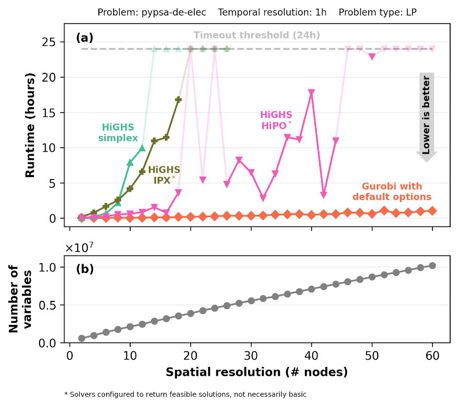
Figure 1: Solver runtime as a function of spatial resolution on the pypsa-de-elec linear programming problem with 1-hour temporal resolution. Panel (a) shows absolute runtime in hours, with an horizontal line indicating the 24-hour timeout. Panel (b) shows the corresponding growth in the number of variables. Note that while HiGHS-simplex and Gurobi guarantee a basic solution, in our setup HiGHS-IPX and HiGHS-HiPO dynamically choose whether to run crossover and may return a feasible (non-basic) solution (see the Appendix for details).

How does HiPO perform on other modelling frameworks?

The benchmark results show that at smaller scales, solver choice matters little; however, once problems exceed 100k variables, HiGHS-HiPO emerges as the most capable open-source option, significantly extending the frontier of solvable problems.

In terms of solver reliability (Figure 2), HiPO achieves a 85.4% success rate on problems from 100k to 1 million variables (5% more than HiGHS-IPX and 46.5% more than HiGHS-simplex) and maintains a 58.5% success rate on problems from 1 to 10 million variables (4% more than HiGHS-IPX and 41% more than HiGHS-simplex). Beyond this extreme-scale threshold, open-source solvers hit hard computational limits and effectively stop working.

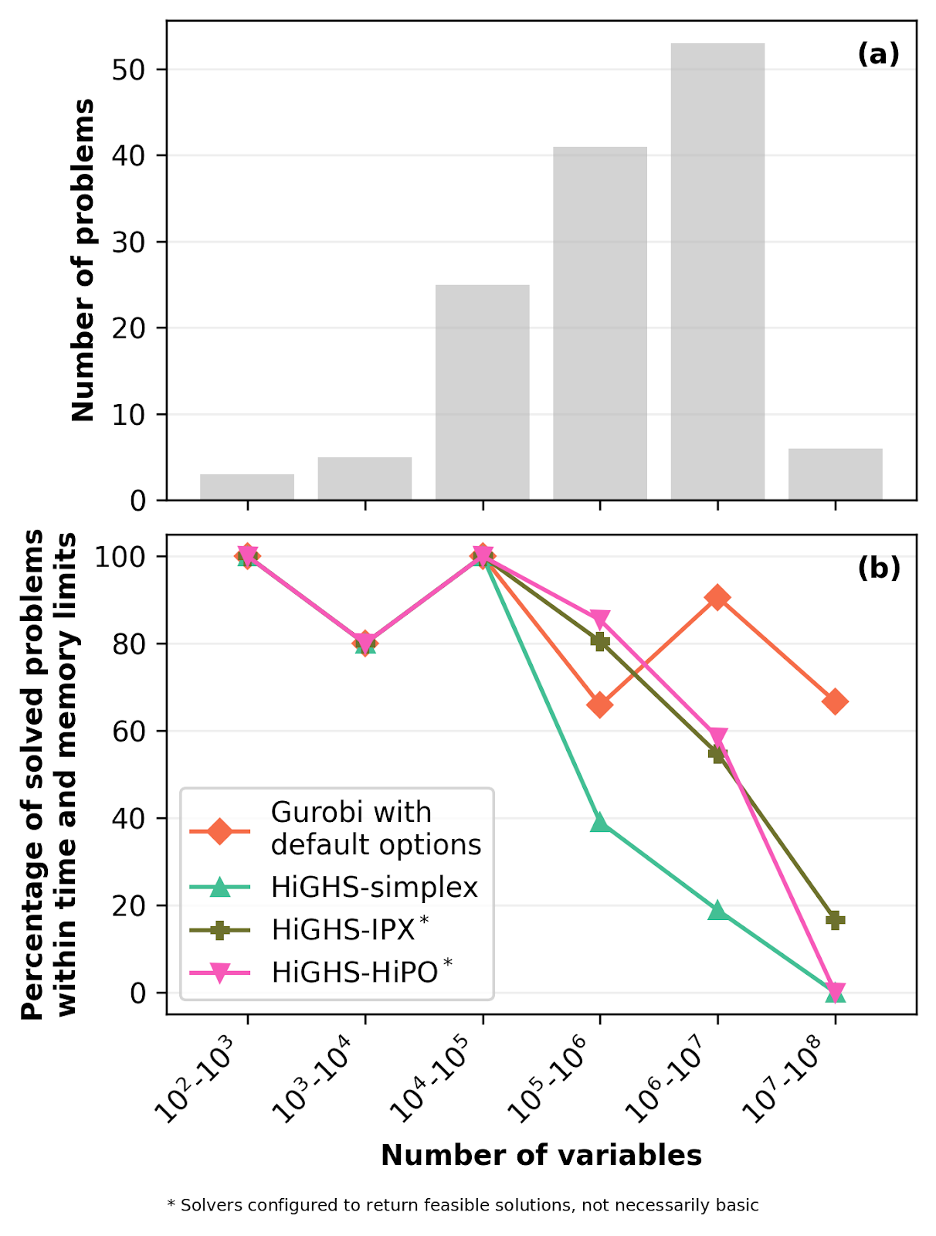
Figure 2: Percentage of successfully solved problems within time and memory limits across different problem sizes (number of variables). Panel (a) shows the absolute number of linear programming problems in each size bin, while panel (b) displays the success rate of each solver configuration. Note that while HiGHS-simplex and Gurobi guarantee a basic solution, in our setup HiGHS-IPX and HiGHS-HiPO dynamically choose whether to run crossover and may return a feasible (non-basic) solution (see the Appendix for details).

When evaluating average runtimes (Figure 3), HiGHS-HiPO clearly emerges as the fastest open-source option for scaling up. While absolute time differences are negligible for models under 100k variables, HiGHS-HiPO decisively pulls ahead as problems grow, running on average up to 4.8 times faster than HiGHS-simplex and up to 96% faster than HiGHS-IPX on models between 100k and 10 million variables. However, at the extreme scale (over 10 million variables), all open-source solvers hit hard computational walls, highlighting the crucial gap that future open-source algorithmic improvements will need to bridge.

It is important to note that the average runtimes reported here are calculated using a shifted geometric mean, where unsolved problems (timeouts and errors) are penalized with a duration equal to twice the time limit. Therefore, at larger scales, a higher average runtime reflects both slower execution and a higher frequency of failure within time limits.

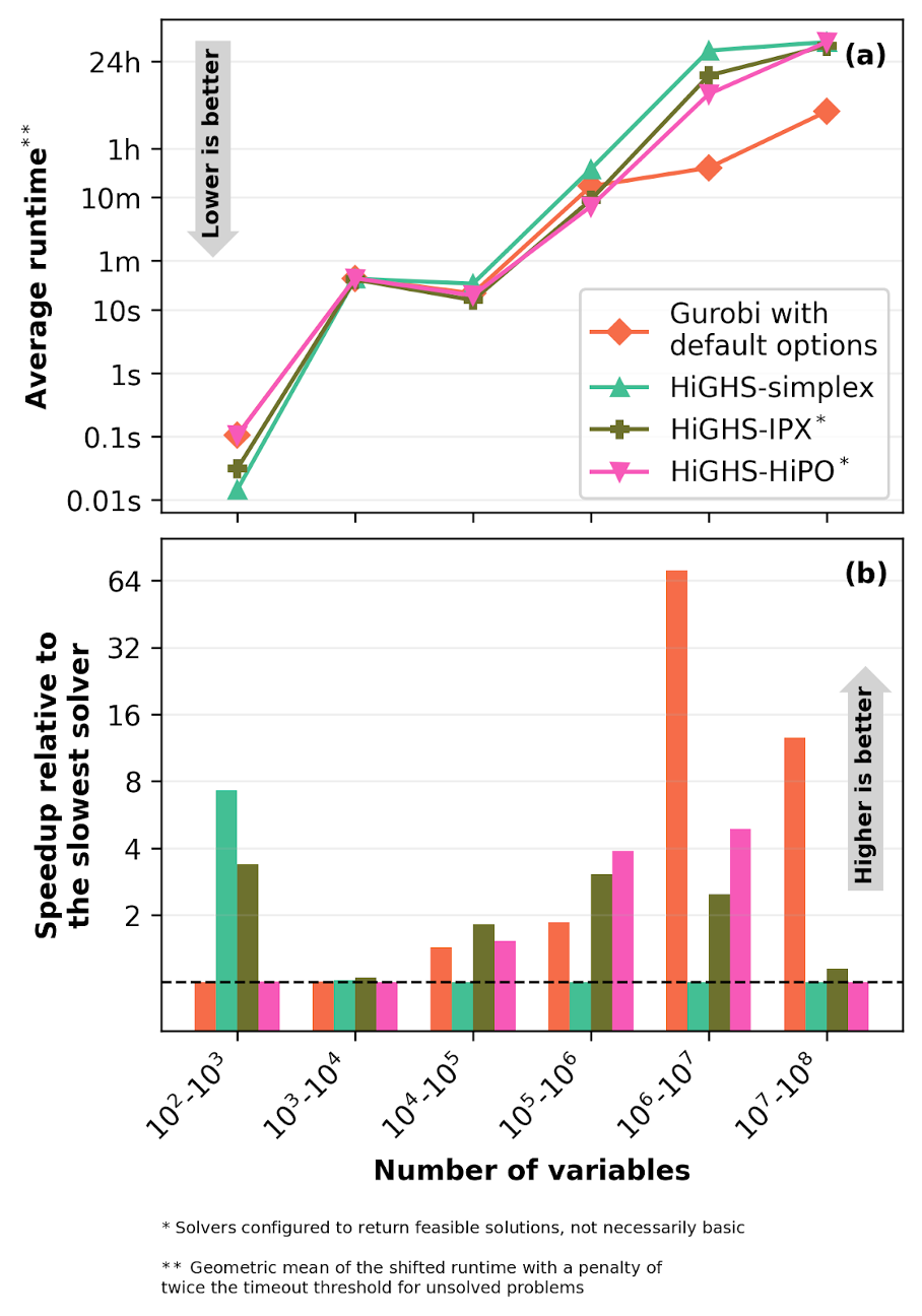
Figure 3: Average runtime scaling across different problem sizes. Panel (a) displays the absolute average runtime in each size bin. This is calculated as the geometric mean of the shifted runtime with a penalty of twice the timeout threshold for unsolved problems. Panel (b) illustrates the relative speed of each solver compared to the slowest solver in that specific size bin (indicated by the dashed line at 1). Note that while HiGHS-simplex and Gurobi guarantee a basic solution, HiGHS-IPX and HiGHS-HiPO dynamically choose whether to run crossover and may return a feasible (non-basic) solution (see the Appendix for details).

Conclusions

The introduction of HiPO represents a meaningful improvement for the open-source solver ecosystem, particularly for energy system modelers. Based on our benchmarking across multiple modeling frameworks, the key takeaways are:

• Extended reach for open-source solvers: HiPO increases the scale of models that can be solved without proprietary licenses. While classical simplex and interior-point methods consistently struggle or time out between 100k and 10 million variables, HiPO successfully solves an additional 4% to 5% of problems in this regime.
• Improved speed at large scale: For problems between 100k and 10 million variables, HiPO provides noticeable performance benefits. It typically solves these large-scale models up to 53 times faster than the default HiGHS-simplex, and up to 15 times faster than HiGHS-IPX.
• More practical modeling in a single day: The combination of increased reach and faster execution means that complex, high-resolution scenarios (such as a 50-node PyPSA Germany electricity model with a 1h time resolution) can now be reliably solved within a standard 24-hour window using purely open-source tools. Previously, these models would frequently hit timeout limits when using classical open-source solvers.

Overall, HiPO is an exciting addition to the HiGHS solver that expands the frontier of what open-source optimization can handle. It allows energy system modelers to run larger, more detailed scenarios than before, significantly lowering the barrier to entry for high-resolution modelling. However, users modeling at the extreme scale—such as highly detailed, sector-coupled models spanning multiple years—will still need to rely on proprietary software such as Gurobi.

Call to action for solver developers

To that end, we want to issue a call to action to the broader open solver development community: the extreme-scale models characteristic of modern energy system planning present a unique and pressing mathematical challenge. We encourage developers to use our open repository to test and improve algorithmic performance to solve those challenging problems.

If you would like to explore these models or test them with your own solver configurations, you can access the problem files below:

• Link to the pypsa-de-elec instances used in the section “What is the largest PyPSA model…”
• Link to the complete set of benchmark instances used in the section “How does HiPO perform…”.
• List of links to the extreme-scale (>10 million variables) problems:
  • genx-elec_co2 (15-168h)
  • genx-elec_trex (15-168h)
  • genx-elec_trex_co2 (15-168h)
  • pypsa-de-sec-trex_copt (50-1h)
  • pypsa-de-sec-trex_vopt (50-1h)
  • SWITCH-China-open-model (32-433ts)

Where can I learn more?

The results from the section “What is the largest PyPSA model…” can be downloaded in full here, and log files (except Gurobi logs that we cannot publish) are available here.

The results presented in the section “How does HiPO perform…” are from the full v2 benchmark dataset. If you want to dive deeper into the data or see how these solvers perform on a specific modelling framework, all results are publicly available on the Open Energy Benchmark website. Users can interactively explore the data across various dashboards, including:

• Benchmark Set: Browse the full list of included problems and their characteristics, and view how solvers performed on any given instance.
• Solvers: Compare the relative performance of a solver to any or all other solvers on any subset of problems.
• Compare Solvers: Compare the runtime and memory usage of any two solvers on any subset of problems.

Where does HiGHS go next and how can we support it?

Following the release of HiPO, the HiGHS development team will now analyze its behavior on this benchmark problem set to guide ongoing performance enhancements. The Open Energy Benchmark will actively support this effort by benchmarking future versions, continuing a highly successful feedback loop between energy modelers and solver developers. The wider modeling community can directly contribute to this process by submitting new benchmark problems—especially extremely large or mathematically challenging ones—to help stress-test the solver at its limits. Finally, because these critical open-source advancements rely heavily on community funding, we strongly encourage users and institutions to support the HiGHS team financially via their GitHub Sponsors page or the Linux Foundation.

Thanks

This investigation and analysis was performed by a team from Open Energy Transition: Enrico Antonini, Jacek Bendig, Kristijan Faust, Fabrizio Finozzi, Siddharth Krishna, Daniele Lerede, and Madhukar Mishra. We are grateful to the HiGHS team for their support with installing and configuring HiPO. We also thank the following collaborators for their thoughtful review and feedback: Oscar Dowson, Ivet Galabova, Julian Hall, Lennart Lahrs, Matthias Miltenberger, Maximillian Parzen, and Mark Turner.

Appendix

Experiment setup

To evaluate the performance of HiPO, we selected different solvers and configurations, namely:

1. HiGHS-simplex: the default simplex algorithm within HiGHS. (Options: random_seed=0.)
2. HiGHS-IPX: the previous implementation of the interior point method within HiGHS and optionally crossover. (Options: random_seed=0, solver=ipx, run_crossover=choose.)
3. HiGHS-HIPO: the new implementation interior point method within HiGHS and optionally crossover. (Options: random_seed=0, solver=hipo, run_crossover=choose, hipo_block_size=64, hipo_metis_no2hop=true.)
4. Gurobi: a reference proprietary software with default options except seed=0.

At present, HiPO must be explicitly enabled through the solver options. According to the HiGHS developers, an upcoming release later this year will run HiPO automatically when it is beneficial.

We benchmarked these solvers configurations on 133 linear programming problems available on the Open Energy Benchmark platform, spanning 13 different modelling frameworks. Together, these problems cover a wide range of objective functions, spatial and temporal resolutions, sectoral scope, investment horizons, and emissions constraints, providing a realistic stress test across both model structure and scale.

All benchmark experiments were executed on Google Cloud virtual machines:

• Problems with fewer than 1 million variables included in the general results were run on c4-standard-2 instances (2 vCPUs, 7.5 GB RAM) with a 1-hour timeout.
• Problems with more than 1 million variables included in the general results were run on c4-highmem-16 instances (16 vCPUs, 128 GB RAM) with a 24-hour timeout.
• Problems in the section “What is the largest PyPSA model…” were run on c4-standard-8 instances (8 vCPU, 30 GB) with a 24-hour timeout.

The experiments described in this blog post commenced in December 2025, prior to any HiGHS release on PyPI or conda-forge that included HiPO. Thus we built HiGHS from source using commit 9e8322a (Nov 26, 2025) and the build steps recommended by the developers (more details here). The default HiGHS configuration (HiGHS-simplex) was version 1.12.0 from conda-forge.

Solution quality: basic vs. feasible solutions

When evaluating solver performance, it is important to consider the type of mathematical solution obtained as well as raw speed. Linear programming solvers typically yield either "basic" or "feasible" (not necessarily basic) solutions, depending on the underlying algorithm.

The simplex method—currently the default in HiGHS—navigates the edges of the problem's feasible region, mathematically guaranteeing a basic (vertex) solution. Basic solutions are widely preferred in optimization because they provide clean, unambiguous dual values.

In contrast, interior-point methods like IPX and HiPO take a path through the interior of the feasible region. This typically allows them to solve problems much faster, but they do not usually converge on a basic solution. To provide a basic solution, interior-point solvers must perform a mathematical procedure called "crossover" after reaching optimality, which can be computationally expensive. However, in our experience, most energy modelling applications do not strictly require a basic solution, allowing modellers to save significant time by disabling crossover.

For this benchmark, because we tested a pre-release version of HiGHS, we allowed the solver to dynamically choose whether to run a crossover. This fallback mechanism was necessary to avoid solver failures: if the interior-point method could not find a solution of sufficient numerical quality, the solver would automatically execute crossover to clean it up and return a valid solution rather than crashing. Future releases of HiGHS are expected to improve the HiPO implementation, making this crossover cleanup unnecessary. Because of this internal heuristic, it is not known a priori whether the solver will ultimately return a basic or feasible solution.

Gurobi’s default setting runs multiple algorithms (simplex and interior-point with crossover) concurrently in parallel. If the interior-point method reaches optimality first, Gurobi automatically performs crossover, ensuring that the solver always returns a basic solution. Users can relax this restriction and allow Gurobi to return non-basic solutions by setting SolutionTarget=1.

Because of these differences, users must be cautious when comparing performance metrics across different solver configurations, as comparing a basic solution with a feasible one is not strictly an apples-to-apples comparison. Nevertheless, we intentionally include these diverse configurations in this benchmark analysis to demonstrate the performance gains possible with HiPO, highlighting the significant step forward it represents for the open-source solver ecosystem.

Investigating the time outs

The performance variability and the time outs for the 20 and 24 node cases of the pypsa-de-elec problem solved with HiGHS-HiPO deserve further investigation. When unusual results occur, there is a lot to be learned by looking at the solution logs (20 node case, 24 node case).

By looking at the 20 node case, the first thing to pay attention to is the coefficient ranges (and associated warnings) that HiGHS prints at the start of each solve:

Coefficient ranges:
  Matrix  \[1e-02, 4e+01\]
  Cost    \[9e-03, 3e+05\]
  Bound   \[1e+10, 1e+10\]
  RHS     \[3e-02, 1e+05\]
WARNING: Problem has some excessively large column bounds
WARNING:    Consider scaling the    bounds by 1e-5, or setting the user\_bound\_scale option to \-14

For this model, HiGHS is telling us that the column bounds are poorly scaled. In fact, all non-zero variable bounds are on the order of 1010. In a modeling context, this means having a decision variable measured in Watts, with a bound on the order of 10s of Gigawatts. HiGHS’s suggestion is that we scale the relevant bounds by 10-5, which would mean re-scaling the relevant decision variables to have units of 0.1 MW instead of W. (It might also make sense to scale by 10-6 to make the units MW.)

The logs show that HiPO runs for 100 iterations before giving up. This is the final iteration that it prints:

 iter       primal obj         dual obj       pinf       dinf       gap    time
  100   5.69287066e+09   5.68614174e+09   3.02e-06   6.71e-09  1.18e-03  2461.8

The optimality gap (the “gap” column) is still on the order of 10-3, which does not meet the tolerance for declaring optimality. To try and improve the gap, HiGHS restarts solving, this time using IPX (“Restarting with IPX” in the logs). (Yes, even though we specified solver=hipo, HiGHS may run multiple solvers in an attempt to find a solution!). IPX runs for 1500 seconds before it too gives up, reporting “IPX reports: ipm no progress”.

As a final attempt to solve the problem, HiGHS tries the simplex solver (“WARNING: IPM solution is imprecise, so clean up with simplex”). This times out, which makes sense because we see HiGHS-simplex times out on smaller problem sizes in our study.

What can you do if you see such warnings?

Solver developers tell us that poor problem scaling is the most common root cause of volatile solve time. Their recommendation is in these cases to either try setting the HiGHS scaling options recommended in the logs, or to modify the model code (in this case PyPSA) to use different units to ensure that variables and bounds have similar orders of magnitude. We hope to investigate the performance of solvers on scaled versions of these models in a future study.

If HiGHS can identify the issue and print a suggested fix, why don’t they apply that by default? Their answer was technical, and it related to the solver’s feasibility tolerance: if they automatically scale the user’s problem, solve it to the given feasibility tolerance, and then un-scale the solution, the final solution might violate the feasibility tolerance. HiGHS developers are therefore investigating changes they could make inside the solver that would improve its robustness to poorly scaled problems like the one in this case study.